Benchmarking Outlier Detection Models for Enterprise AI

TL;DR: Benchmarking outlier detection helps enterprise teams choose anomaly detection models with evidence instead of guesswork. Strong benchmarks use representative datasets, fair protocols, clear metrics, reproducible tuning, and production efficiency checks. The goal is to select models that perform reliably in real operating conditions, not just on paper.

Benchmarking Outlier Detection: Why It Matters for Enterprise AI Decisions

Benchmarking outlier detection means testing multiple anomaly detection methods under identical conditions so you can compare results fairly. That matters because teams often need more than a score. They need to determine which outliers are being detected, how stable the results are, and whether the method can handle real data without creating too many false alarms.

Enterprise teams usually do not struggle because they cannot find an outlier detection method. They struggle because the wrong model can look perfectly convincing right up until it hits production. A missed outlier can hide fraud, equipment failure, or a bad estimate. Too many false alarms can bury teams in noise and quickly erode trust in the AI stack.

That pressure is only growing as bids get tighter, projects span more systems, and decision data becomes harder to reconcile. In estimation-heavy environments, cost estimation software such as CostOS can create a more structured foundation, but model selection still depends on knowing which outlier detection techniques can be trusted under realistic conditions.

This article explains how rigorous benchmarking turns outlier detection from a risky model choice into defensible decision evidence. Use it to understand what strong benchmarks measure, where common comparisons go wrong, and how to choose models with more confidence before they affect live operations.

Turning Algorithm Comparisons Into Business-Ready Evidence

When a team needs to justify an AI investment or choose an outlier detection method for a critical pipeline, raw algorithm comparison rarely tells the whole story. What matters is how those benchmarks were built and what they actually measured.

That is where systematic benchmarking frameworks become useful. Research like ADBench is a strong example of disciplined comparison in practice. The paper evaluated 30 anomaly detection algorithms across 57 benchmark datasets covering tabular data, images, and text. Just as important, it standardized preprocessing, evaluation protocols, and performance metrics so every algorithm was tested under the same conditions.

That consistency is what makes the results useful. When benchmarking is handled this way, your team can:

• Compare new or emerging models against a wide set of established baselines
• Know that performance differences reflect real capability gaps, not inconsistent test conditions
• Build a clear, defensible evidence base for model selection

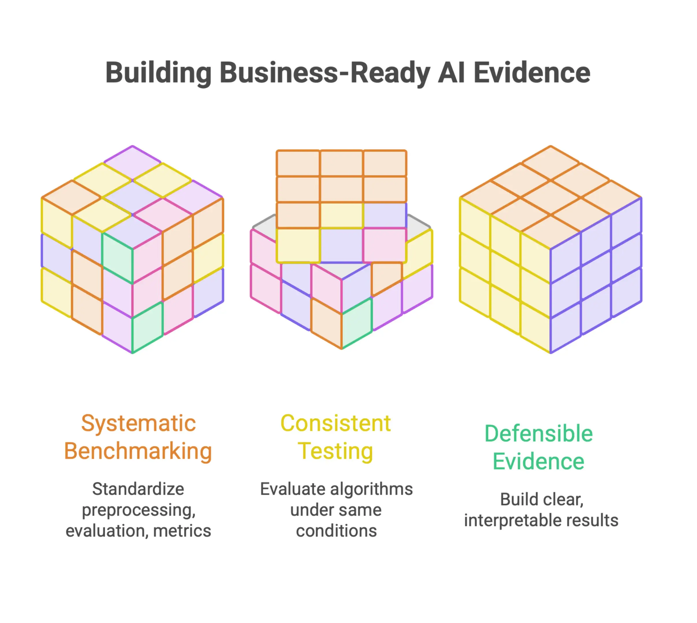
Without that consistency, model comparisons get messy fast. Once the results are hard to interpret, they are even harder to explain to non-technical stakeholders.

Avoiding Misleading Rankings and Overstated Model Performance

One of the biggest blind spots in benchmarking outlier detection is that poor evaluation data can make a weak model look impressive. This is not a theoretical concern. It is a known issue, and it can distort how models are ranked and selected.

Research published through the IEEE Computer Society examined widely used anomaly detection benchmarks and found structural flaws that skew evaluation results. The authors identified four categories of issues in existing benchmarks, including mislabeled anomalies and detection cases so obvious that nearly any algorithm would pass them. Problems like these directly affect rankings. If an organization relies on those rankings to guide selection, it may end up choosing a model that performs well on a flawed benchmark but fails in the field.

The research points to a simple but important fix: better curation. By creating an archive of 250 carefully vetted time series anomaly exemplars, the authors showed that benchmark quality matters just as much as benchmark volume.

For enterprise teams, the takeaway is straightforward. Before trusting a published comparison, ask:

• Were the benchmark datasets properly labeled and validated?
• Does the evaluation include realistic edge cases, or only easy detection scenarios?
• Are the rankings stable across multiple datasets, or do they depend on a narrow test set?

Those questions help keep high-stakes decisions from being shaped by inflated claims.

Matching Benchmarking Strategy to Stakeholder Needs

Not everyone evaluating anomaly detection models is looking for the same answer. A data scientist wants to know which algorithm generalizes best across data types. An operations manager wants fewer false positives in a specific workflow. A risk officer wants confidence that the chosen approach has been tested against realistic failure modes.

A benchmarking strategy that works well for one group can easily miss what another group actually needs. That is why stakeholder context matters just as much as technical rigor.

The multi-dataset approach used in frameworks like ADBench is useful here. By evaluating algorithms across tabular, image, and text datasets within one consistent framework, it becomes easier to share findings in a way each audience can use. A team working with structured transactional data can focus on tabular results. A team building computer vision workflows can lean on the image findings. Both are still working from the same methodologically sound evaluation.

Aligning benchmarking with stakeholder needs also means being honest about what a benchmark can and cannot prove. Published results on curated datasets are a starting point, not the final word. They give you a foundation for deeper testing on your own data and in your own operating environment.

When benchmarking outlier detection is treated as a structured, stakeholder-aware process instead of a one-off model comparison, it becomes a real decision-support tool. That is the difference between AI adoption that creates value and AI adoption that quietly introduces new risk.

Benchmark Dataset Design: Building Fair and Representative Test Beds

Designing a reliable benchmark for outlier detection is harder than it looks. Dataset selection, anomaly mix, and labeling quality all shape the conclusions you can actually trust. A benchmark that works well in one domain, or for one algorithm family, can give a misleading picture somewhere else. If you want a test bed that stands up to scrutiny, you need to think about diversity, coverage, and curation from the start.

Using Large-Scale Tabular Benchmarks for Real-World and Synthetic Outliers

When you evaluate tabular outlier detection methods, scale and variety matter. A benchmark built on only a few similar datasets tends to reward methods that happen to fit those specific data characteristics. That makes the results hard to generalize.

The MacrOData paper on arXiv tackles this directly with a benchmark suite built from 2,446 datasets across three components. The first, OddBench, includes 790 datasets focused on real-world semantic anomalies. The second, OvRBench, includes 856 datasets centered on real-world statistical outliers. The third, SynBench, adds 800 synthetic datasets designed to cover a broad range of data priors and outlier archetypes. Together, these components keep any single anomaly type or data distribution from dominating the evaluation.

The authors also provide an open-source leaderboard, and that matters for more than tidy reporting. Methods such as cluster analysis are also useful here because they can detect unusual data clusters in large datasets. It creates a consistent way to compare methods across a large corpus, which reduces the risk of cherry-picked results or inconsistent test setups. For teams building or reviewing outlier detection pipelines, that kind of structured benchmark is much stronger than a small, ad hoc evaluation.

How CosMO Applies Outlier Detection to Cost Benchmarking

Cost benchmarking provides a practical example of why representative datasets and careful outlier analysis matter. In CosMO, statistical screening helps cost professionals identify historical projects that may require further investigation before they are included in a benchmark.

One of the most important yet often underestimated steps in cost benchmarking is deciding which historical projects genuinely belong in the benchmark population. Historical databases inevitably contain projects that sit far outside the normal range, such as an unusually expensive project, an exceptionally low bid, a project delivered under abnormal market conditions or a record affected by incomplete or inconsistent data. Including such observations without examination can significantly distort averages, cost relationships and ultimately the conclusions drawn from a benchmark.

This is why CoSMO applies statistical outlier detection as part of the benchmarking process rather than relying solely on visual judgement. The principle follows established cost-engineering practice: before historical data is used to establish a benchmark, it should be normalized and examined for observations that are not representative of the population being analysed. AACE guidance similarly stresses the importance of ensuring that datasets used for cost analysis are free from significant unexplained outliers that could bias the resulting analysis.

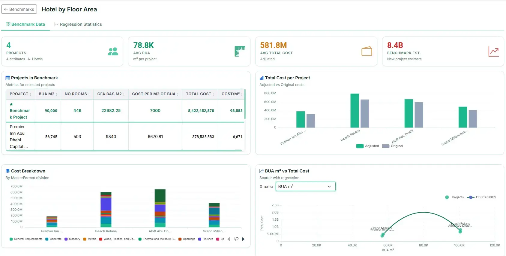
The important word, however, is “unexplained.” An outlier is not automatically bad data. A project may be statistically unusual because there is a perfectly legitimate engineering or commercial reason behind it: exceptional ground conditions, remote logistics, acceleration, unusually high specifications, a different contracting strategy or a sudden shift in market prices. Consequently, CoSMO’s statistical screening should be seen as a mechanism for identifying projects that require investigation, rather than blindly deleting data simply because it is distant from the mean.

This distinction becomes particularly important when benchmarking relatively small groups of comparable projects. A single extreme value can materially change the calculated average, cost per unit, regression relationship or expected cost range. Removing a genuine anomaly can therefore make the benchmark significantly more representative, while incorrectly removing a legitimate project can make the benchmark artificially narrow. Effective benchmarking combines the statistical test with engineering judgement, project classification and appropriate normalization for factors such as location, currency, time and scope.

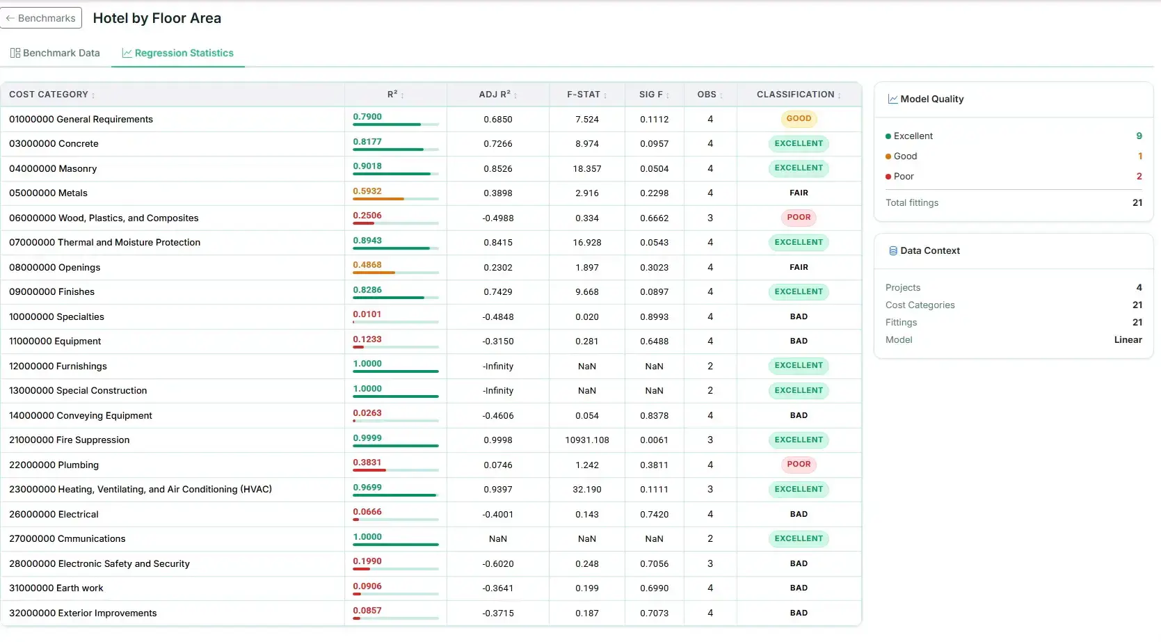
Ultimately, the objective is not to produce the cleanest-looking dataset; it is to produce the most representative benchmark. CoSMO uses the available historical population, normalization techniques and statistical analysis together to highlight observations that warrant attention and allow the cost professional to decide whether they should remain part of the benchmark set. In this way, outlier management becomes an auditable part of the benchmarking process—helping turn a collection of historical project costs into a more reliable basis for estimating, validation and decision-making.

Curating Time Series Benchmarks to Reflect Real Detection Challenges

Time series anomaly detection comes with its own complications. Outliers can be point-level, contextual, or pattern-based, and the temporal structure of the data introduces evaluation issues that do not show up in tabular settings.

A 2023 survey referenced by HAL-Inria examines how benchmark design choices shape reported performance across the time series space. It highlights TSB-AD as a strong benchmark suite, built around a heterogeneous, curated collection of anomaly detection datasets and a more complete evaluation setup. The survey also compares several other well-known benchmarks, including UCR, TODS, TimeEval, TSB-UAD, and TimeSeAd, and it lays out details such as dataset count, whether the series are univariate or multivariate, which algorithm families are included, and what evaluation measures are used.

That comparison makes one thing clear: benchmark design is never neutral. The choices baked into a benchmark directly affect which algorithms look strong and which do not. For example, a benchmark built only on univariate series will naturally favor methods that were never meant to capture dependencies across channels. Good time series benchmark curation means paying attention to those structural details, not just adding more data.

Balancing Synthetic, Semi-Synthetic, and Real-World Anomalies in Simulation Study

One of the most important decisions in benchmark design is how to balance anomaly sources. Each option brings trade-offs that affect how useful and how credible your evaluation really is.

Real-world outliers are the most relevant, but they are also the messiest. Labels can be noisy, anomaly rates are often extremely low, and the root cause is not always obvious. Synthetic outliers give you tight control over what an anomaly looks like and make it easier to cover edge cases systematically, but they can look too clean compared with what actually appears in production.

The MacrOData benchmark is a good example of how to handle that tension deliberately. It brings all three types into one structured suite. OddBench and OvRBench cover real-world anomalies at scale, while SynBench adds synthetic data that spans a wide range of data priors and outlier archetypes. That mix helps researchers separate generalization on real data from performance on controlled anomaly types.

The same issue shows up in time series evaluation. As the HAL-Inria survey shows, different benchmarks make different composition choices, and those choices clearly shape the performance landscape. A benchmark that leans too heavily on synthetic data may produce rankings that look tidy and stable but do a poor job predicting how a method will behave on noisy real-world signals.

The practical takeaway is simple: a strong benchmark does not rely on just one anomaly source. It includes enough variety across synthetic, semi-synthetic, and real-world examples to reveal both the strengths and the blind spots of the methods being tested.

Evaluation Protocols and Metrics: Measuring What Actually Matters

Getting outlier detection to work in a controlled experiment is one thing. Getting it to hold up in production is another. The gap often comes down to how performance is measured from the start. Use the wrong metrics, apply loose labeling rules, or ignore the cost of different error types, and you end up with benchmark results that look great on paper but fall apart in practice. This section looks at the evaluation choices that separate useful benchmarks from misleading ones.

Comparing Detection Accuracy Metrics Across Time Series Benchmarks

Not all accuracy metrics tell the same story. Comparing results across benchmarks without understanding what each metric captures is a quick way to pick the wrong model.

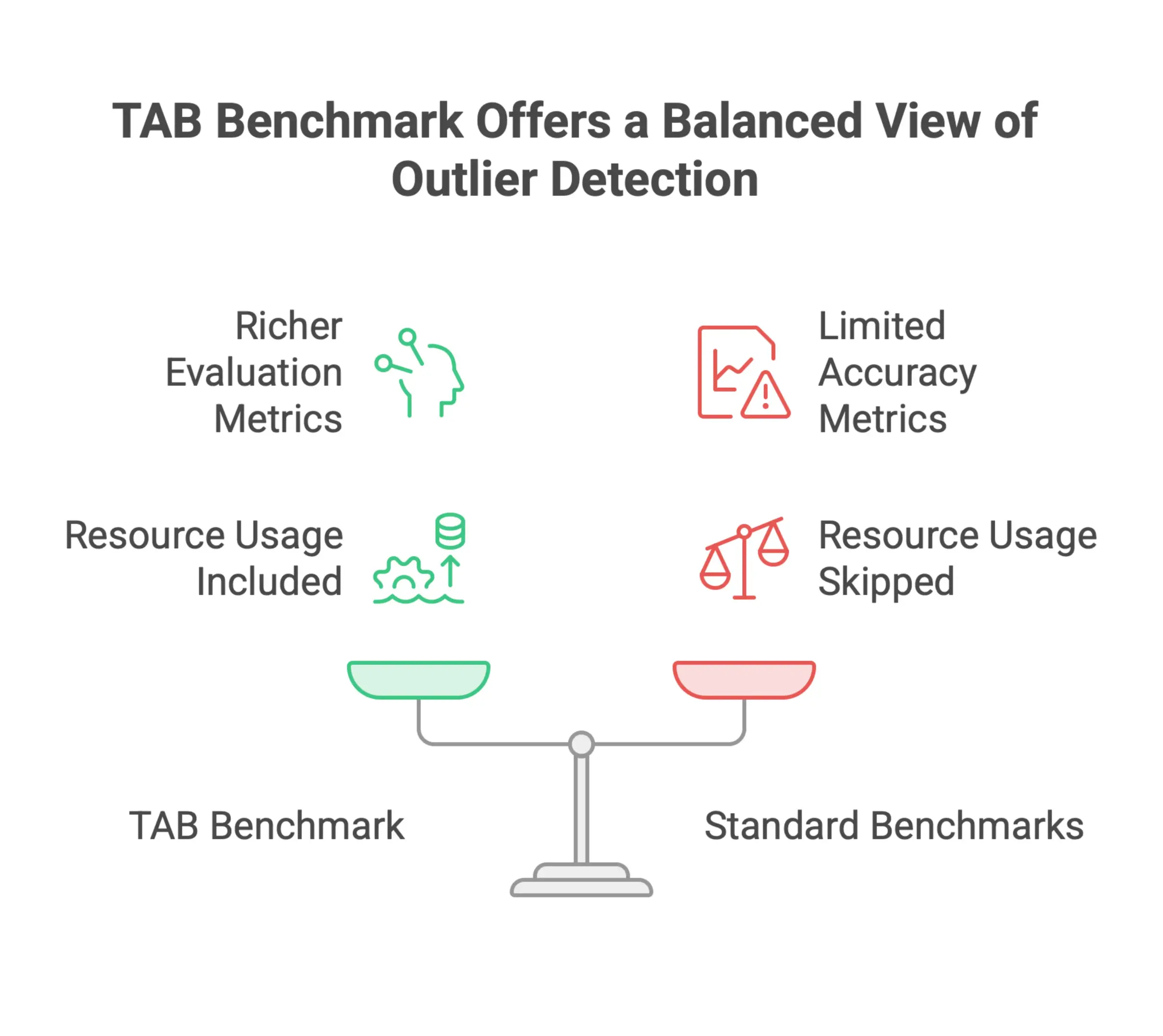
A number of benchmarks are moving toward richer evaluation frameworks for exactly this reason. The TAB benchmark is a good example. It evaluates 48 anomaly detection methods across 29 multivariate datasets and 1,635 univariate time series, using metrics that go well beyond standard precision and recall. It reports both Affiliated-F1 and VUS-PR, which gives a more complete picture of how well a method detects outliers across different thresholds and alignment conditions. Just as importantly, TAB also includes resource usage, with CPU and GPU time plus memory consumption, so accuracy is always viewed alongside computational cost.

That distinction matters. A method that scores a little better on Affiliated-F1 but uses three times the compute may not be the right choice for a latency-sensitive deployment. Benchmarks that reduce everything to a single accuracy number leave out the context you need to make a sound decision.

When comparing results across different benchmarks, watch for these common mismatches:

• Metrics that reward partial detections differently
• Benchmarks that combine performance across domains without showing domain-level results
• Studies that skip threshold sensitivity analysis altogether

Applying Strict Detection Windows and Label Rules

How a benchmark defines a correct detection can have a bigger impact on final scores than most teams expect. Loose labeling rules can make methods look stronger than they really are.

The Expert Systems (Wiley) benchmarking study on the UCR Time Series Anomaly Archive uses a strict rule: a prediction only counts if it lands inside the labeled anomaly segment itself. There is no buffer zone and no partial credit for near misses. Performance is measured as the share of time series where anomalies are correctly detected. Under this protocol, DeepSVDD came out as the top-performing method across all reported metrics.

That kind of window-based evaluation deserves attention. It forces methods to be precise, not just roughly correct. It also makes results easier to reproduce, since there is no ambiguity about what counts as a hit.

When choosing or designing a benchmark protocol, consider:

• Whether detection windows are fixed by the dataset or adjustable by the researcher
• How the protocol handles anomalies that span multiple time steps
• Whether the same labeling rules apply consistently across all methods being compared
• Whether results are evaluated at the level of each instance, not only aggregate detections

Inconsistent label rules across methods are one of the most common reasons published benchmarks end up being unfair.

Choosing Metrics by Business Cost: False Positives, False Negatives, and Latency

Technical accuracy metrics are only the starting point. The metrics that matter most in production depend on what each type of error actually costs the business.

A false positive in a fraud detection pipeline might trigger a customer service call. In a manufacturing environment, it might stop a production line for no good reason. A false negative in a network intrusion system could leave a breach undetected for hours. Those are very different failures, and poor metric choices can lead teams to predict the wrong operational tradeoff, so your evaluation protocol should treat them that way. Even a simple baseline like z-score analysis measures how many standard deviations a value is from the mean, which helps clarify how threshold choices map to business cost.

The TAB benchmark takes a useful step in this direction by testing methods in zero-shot, few-shot, and full-shot settings while also reporting efficiency metrics. That lets teams judge not just accuracy, but speed and infrastructure demand as well. For time-sensitive use cases, a method with slightly lower precision but much lower latency may be the better operational choice.

In practice, aligning evaluation with business cost means:

• Defining acceptable false positive rates before choosing a method
• Weighting precision and recall based on the operational impact of each error type
• Including detection latency as a core metric when real-time monitoring is involved
• Testing across multiple regimes, as TAB does, to see how performance changes when labeled data is limited

A benchmark that ignores these tradeoffs will keep steering teams toward methods that optimize a score instead of the outcome that actually matters. The real goal of any evaluation protocol is to make lab results a realistic proxy for production behavior.

Hyperparameter Tuning and Reproducibility: Making Benchmark Results Trustworthy

Benchmarking outlier detection algorithms sounds simple enough: run a few methods across a set of datasets, compare the scores, and pick a winner. In reality, the outcome depends heavily on how those experiments are run. Hyperparameter choices, preprocessing steps, and reporting habits can all move the rankings around in ways that have little to do with the algorithms themselves. If you want benchmark results you can trust and actually use, reproducibility and experimental control are not optional. They are the baseline.

Why Per-Dataset Hyperparameter Optimization Changes the Leaderboard

One of the easiest ways to distort benchmark results is to use the same default parameters for every dataset within an algorithm. It feels consistent, but it quietly introduces bias. Good algorithms can look underwhelming, and weaker ones can seem more competitive than they really are.

Research published on IEEE Xplore shows this clearly. A 2024 simulation study benchmarking 34 anomaly detection methods found that the best hyperparameter settings varied a lot from one dataset to another, even for the same algorithm. Once per-dataset tuning was applied consistently, the rankings changed in meaningful ways. Without that step, the comparisons were misleading.

The lesson for anyone building or reading benchmarks is straightforward: you cannot judge an algorithm fairly using default parameters or settings tuned for some other dataset. You only see what an algorithm can really do when it gets a fair chance on the data it is actually being tested against.

The practical takeaway is just as clear. Benchmark reports should document not only which hyperparameters were used, but how they were chosen. Was there a search process? What range was explored? Was the same tuning method used across all algorithms? Those details tell you whether you are comparing methods or just comparing assumptions.

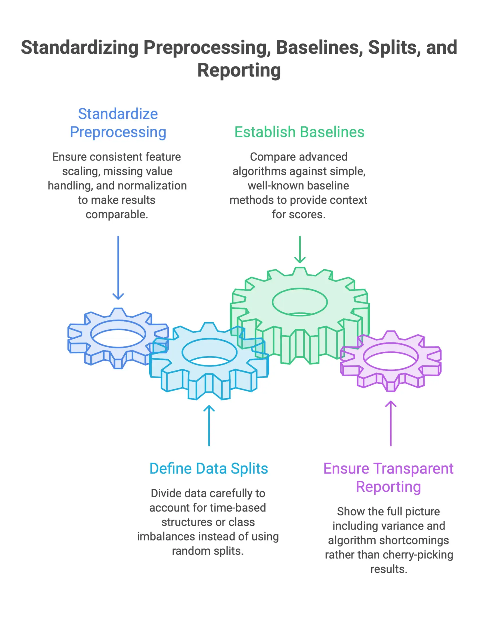
Standardizing Preprocessing, Baselines, Splits, and Reporting

Hyperparameter tuning is only one part of reproducibility. Even with careful tuning, benchmark results can drift in ways that are hard to explain if the rest of the setup is not consistent.

A few areas matter a lot:

• Preprocessing: Feature scaling, missing value handling, and normalization all affect how anomaly detection techniques behave. If two studies preprocess the same dataset differently, their results are not truly comparable, even if they use the same algorithms.
• Train and test splits: How the data is divided matters, especially when the dataset has time-based structure or class imbalance. Random splits that ignore those patterns can make metrics look better or worse for reasons that have nothing to do with model quality.
• Baselines: A result only means something when it is compared against a reference point. Including simple, well-known baseline methods alongside more advanced algorithms helps readers understand what the reported score actually represents.
• Reporting: Averaging results across datasets without showing variance, or choosing which datasets to include only after seeing the outcomes, makes a benchmark look cleaner than it really is. Transparent reporting means showing the full picture, including where an algorithm falls short.

The IEEE Xplore study reinforces why this matters. By using a structured optimization process across all 34 algorithms and multiple datasets, the researchers created a setup where methods could be compared on equal footing. That kind of consistency is what separates a trustworthy benchmark from one that mostly confirms what people expected to see.

Using Open Leaderboards Without Overfitting to Public Benchmarks

Open leaderboards and shared benchmark datasets have made it much easier to track progress in anomaly detection research. They give teams a common frame of reference and help identify methods that hold up across datasets. Used well, they are valuable.

The catch is a subtle kind of overfitting that happens at the research level, not just inside the model. When an algorithm is tuned and retuned against the same public benchmark, the leaderboard starts measuring familiarity with that benchmark rather than true generalization.

Keep that in mind when interpreting published results. A method sitting at the top of a well-known leaderboard may have been optimized, directly or indirectly, for the quirks of that specific dataset collection. As the IEEE Xplore findings suggest, performance can shift a lot when the evaluation setup changes. An algorithm that looks dominant under one tuning process may look far less convincing when it is tested on a new dataset with fresh optimization, and a small leaderboard gain does not always corresponds to better real-world generalization.

Practical ways to use open leaderboards more responsibly include:

• Treating leaderboard rankings as a starting point, not the final answer
• Testing shortlisted algorithms on internal or held-out datasets that were never part of the public benchmark
• Checking whether top submissions clearly explain their tuning process and preprocessing pipeline to ensure validation steps handle data consistently before comparison
• Focusing on methods that perform steadily across many datasets, not just those that spike on a narrow subset

The goal is to use public benchmarks as a filter, not a finish line. Reproducible, well-controlled experiments on data that reflects your actual use case will always tell you more than a leaderboard rank on its own.

Production Efficiency Benchmarks: Accuracy Is Not Enough

When you evaluate outlier detection models for production, accuracy is only part of the picture. A model can score well on benchmark datasets and still be a poor fit if it uses too much memory, takes too long to run inference, or becomes expensive to maintain. For decision-makers, the real question is broader: how well does the model detect outliers, and what does it actually cost to run at scale?

Some methods look excellent on paper, but these tradeoffs should be considered explicitly for large-scale evaluations, especially when comparing time complexity across methods. This section covers the metrics that matter most when moving from research-style evaluation to production-ready benchmarking.

Benchmarking Training Time, Inference Time, and Memory Consumption

Precision, recall, and AUC are useful starting points, but they do not tell you whether a model can hold up in a live environment. According to arXiv: Benchmarking Anomaly Detection Algorithms, evaluation needs to include resource usage as well as detection quality, especially training time, inference time, and memory consumption; some methods also derive threshold decisions from outlier scores, so efficiency should be judged alongside score quality.

That matters because strong benchmark results do not always translate into workable deployments. Some methods look excellent on paper but become hard to justify once compute demands, latency, and infrastructure overhead enter the picture.

When building your benchmarking framework, measure:

• Training time across different dataset sizes to see how the model scales
• Inference latency under realistic throughput conditions, not just one-sample tests
• Peak memory usage during both training and inference

These measurements give your team the information needed to choose a model that will actually work under production load, not just in a controlled test environment.

Evaluating Zero-Shot, Few-Shot, and Full-Shot Deployment Scenarios

Not every project begins with a clean, fully labeled dataset. In real deployments, teams usually face one of three situations: no labeled examples, a small set of confirmed anomalies, or a complete annotated training set. The same model can behave very differently in each case. Repeated testing across zero-shot, few-shot, and full-shot settings makes the comparison more robust.

That is why benchmarking across these scenarios matters. A model that looks strong in a full-shot setup may struggle when labels are limited. At the same time, lighter methods built for zero-shot use can perform better than expected when labeled data is scarce.

The arXiv paper on benchmarking anomaly detection algorithms makes the case for multi-dimensional evaluation, and that naturally includes testing models under the level of data availability your team will actually have. If you benchmark all three scenarios, you get a clearer view of fit, not just raw performance.

Structure your scenario testing around:

• Zero-shot: Can the model generalize without labeled anomalies?
• Few-shot: How does performance change with five, ten, or twenty labeled examples?
• Full-shot: What does performance look like when full supervision is available?

This kind of testing exposes trade-offs that a single aggregate score will never show.

Connecting Benchmark Results to Total Cost of Ownership

Benchmark results only become useful when they support an actual decision. That means translating model performance into cost terms the business can understand and act on.

Total cost of ownership for an outlier detection system goes well beyond licensing or infrastructure bills. It includes the engineering effort needed to train and retrain models, the compute costs tied to inference at scale, the memory footprint that affects infrastructure sizing, and the operational risk of deploying a model that misses important edge cases.

As highlighted by arXiv: Benchmarking Anomaly Detection Algorithms, models that look strong on accuracy alone can become expensive liabilities in production once compute and operational overhead are included. That is why multi-dimensional benchmarking is not optional. It is part of responsible deployment.

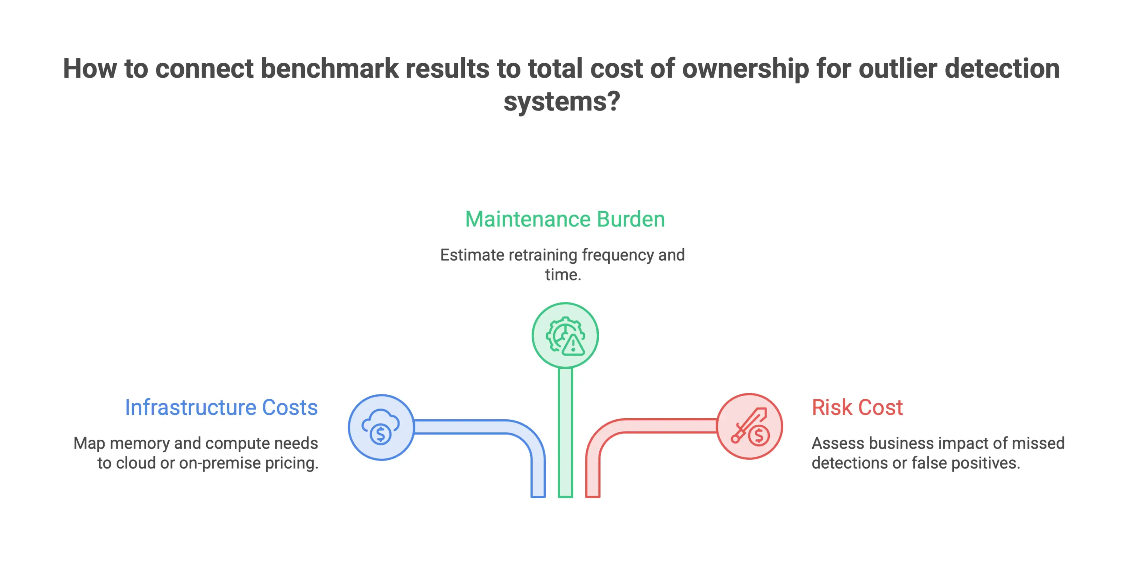
A practical total cost of ownership review should connect benchmark results to:

• Infrastructure costs: Memory and compute needs mapped to cloud or on-premise pricing
• Maintenance burden: How often retraining is needed and how much time it takes
• Risk cost: The business impact of missed detections or false positives in your domain

When benchmark data feeds directly into those calculations, procurement and deployment decisions become much easier to defend. Tools like CostOS can help teams keep those comparisons grounded in operational reality, not just headline accuracy numbers.

Industry-Specific Benchmarks: Matching Methods to Operational Context

Outlier detection is not a one-size-fits-all exercise. The right method depends on the data, the operational risk, and what “anomaly” actually means in that setting. A spike in sensor readings on a chemical line is a very different problem from an unusual movement in surveillance footage or a surface defect on a manufactured part. As a result, benchmarking has evolved differently in each domain, with specialized datasets, metrics, and method rankings that reflect the realities of the environment.

Here is how the benchmarking landscape breaks down across three key industrial and operational contexts.

Industrial Process Monitoring and Chemical Manufacturing

Process industries like chemical manufacturing produce continuous, high-dimensional sensor data, where catching deviations early can prevent expensive failures or safety issues, and those early indicators can lead teams to investigation of faults before they become expensive failures. Benchmarking anomaly detection in this space means using datasets that capture the complexity and interdependence of real industrial systems.

The Tennessee Eastman Process dataset has become a standard reference point here. A large-scale study published in Wiley Online Library (Chemie Ingenieur Technik) benchmarked a wide range of modern unsupervised deep anomaly detection methods against it. The results were clear and useful: reconstruction-based models consistently performed best, with generative and forecasting-based methods following behind.

For chemical and process engineers, that ranking is more than academic. It gives teams a practical place to start instead of scattering effort across every possible method family. If you are evaluating options for a real plant environment, reconstruction-based architectures deserve serious attention first. That is the value of domain-specific benchmarking. It narrows the field based on evidence, not guesswork.

Key considerations when benchmarking in this domain include:

• Whether the benchmark dataset reflects realistic fault distributions and sensor interdependencies
• Whether the evaluation uses unsupervised settings, since labeled fault data is often limited in real plants
• How well methods generalize across different process states and operating conditions

The common thread across all three domains is simple: context shapes everything. It affects the dataset, the metric, the method category, and even how success should be defined. If you borrow benchmarks from a nearby field without accounting for those differences, you can end up with misleading conclusions and the wrong method choice in practice.

Algorithm Families and Outlier Detection Techniques in Outlier Detection Benchmarks: Choosing the Right Baselines

One of the easiest mistakes in anomaly detection is letting a benchmark revolve around a single method. In reality, no algorithm wins everywhere. Performance shifts with the dataset, the domain, and even the type of anomaly you are trying to catch. A solid benchmark pulls from multiple algorithm families so teams can see where each approach is genuinely useful and where it starts to fall apart.

Knowing how these families differ, and when to use each one, is what separates a meaningful evaluation from one that simply reinforces what people already expect to see.

Classical Machine Learning, Non-Learning, and Statistical Baselines

Before moving to more complex models, it is worth setting strong baselines with classical methods. Isolation Forest, Local Outlier Factor, and One-Class SVM have stayed relevant because they are practical. They are easier to interpret, lighter on compute, and their failure modes are generally well understood.

Statistical methods, including Z-score-based techniques, ARIMA residuals, and distribution-fitting approaches, still have a clear place, especially when datasets are smaller or the anomaly pattern is fairly direct. They often make fewer assumptions about structure, which makes them easier to explain and validate with subject matter experts.

Non-learning methods, such as distance-based or density-based detectors, also play an important role in benchmarks because they avoid training bias altogether. If a simple non-learning method beats a trained model on a specific dataset, that is not noise. It usually tells you something important about the data itself.

These baselines should be in every benchmark. They keep the evaluation grounded and make it harder for more complex methods to overstate their value.

Deep Learning, Reconstruction-Based, Generative, and Forecasting Models

Deep learning has broadened the anomaly detection toolkit, especially for high-dimensional and time-dependent data. Reconstruction-based approaches, such as autoencoders and variational autoencoders, work on a simple idea: if a model learns what normal looks like, it should struggle more when something unusual appears. That usually shows up as a higher reconstruction error. In unsupervised settings, where labeled anomalies are limited, that can be a very useful signal.

Generative models, including Generative Adversarial Networks, take a different route. They learn the data distribution itself and then flag inputs that sit outside it. These models can capture complex nonlinear patterns that classical approaches often miss, but they also tend to be harder to train and less stable in practice.

Forecasting models matter most in time series benchmarks. LSTM-based predictors and Transformer-based sequence models identify anomalies as points that drift away from expected future values. That makes them a natural fit for monitoring use cases where timing and sequence matter, such as sensor data, machine telemetry, or transaction streams.

The tradeoff across these deep learning families is consistent. More modeling power usually means more sensitivity to hyperparameters, data quality, and compute requirements. Any benchmark that includes them needs to account for that if it wants to make fair comparisons.

Emerging LLM-Based and Pre-Training Approaches for Anomaly Detection

Large language models and foundation model pre-training are becoming part of the anomaly detection conversation, and for good reason. The idea is straightforward: if a model has already learned from large, varied datasets, it may transfer useful representations into anomaly detection tasks even when task-specific labeled data is limited.

In tabular and log-based detection, LLM-based approaches are especially interesting because they can handle messy, semi-structured inputs that traditional models often struggle with. Instead of building heavy feature engineering pipelines, teams can work more directly with raw descriptions, logs, or mixed-format records. CostOS-style workflows that bring structure to estimation and project data are a good example of where this kind of flexibility can matter.

Pre-training methods more broadly, including contrastive learning and self-supervised approaches, are also gaining traction because they reduce dependence on labeled anomaly examples. That is a big deal in production environments, where anomalies are rare, inconsistent, and expensive to label well.

Still, these methods are early in their maturity curve. Benchmarks that include LLM-based or pre-trained models should be careful about how they evaluate them. Standard metrics and split strategies do not always tell the full story, especially when a model is learning surface patterns rather than real anomaly structure. For now, the right way to treat these approaches is as promising options, not default winners.

How to Build an Outlier Detection Benchmarking Strategy: A Practical Roadmap

Building a benchmarking strategy for outlier detection is not just a technical exercise. It is the framework that guides how your organization chooses tools, governs models, and keeps performance steady once the system is in production. Whether you are comparing vendors, validating a new algorithm, or managing an already deployed model, a clear roadmap keeps everyone aligned and makes each decision easier to defend.

Here is how to build that roadmap from the ground up.

Define the Business Objective, Data Modality, and Risk Tolerance

Before you look at a single algorithm or dataset, anchor the benchmark to a clear business purpose. The point is not to find the “best” outlier detection method in the abstract. It is to find the method that works best for your problem, your data, and your tolerance for being wrong.

Start by asking three basic questions:

• What is the business objective? Are you detecting fraud, catching equipment failure early, spotting data quality issues, or monitoring model inputs for drift? Each use case defines outliers differently, and each one carries a different cost when something slips through.
• What is the data modality? Tabular, time-series, image, text, and graph data all behave differently when anomalies appear. A method that performs well on structured tabular data may struggle with noisy sensor streams or high-dimensional inputs. Your benchmark should match the data your system will actually see.
• What is your risk tolerance? This is where business reality shapes the technical approach. A false negative in fraud detection can mean direct financial loss. A false positive in manufacturing quality control can trigger unnecessary downtime. If you quantify those tradeoffs early, it becomes much easier to choose metrics that actually matter to stakeholders.

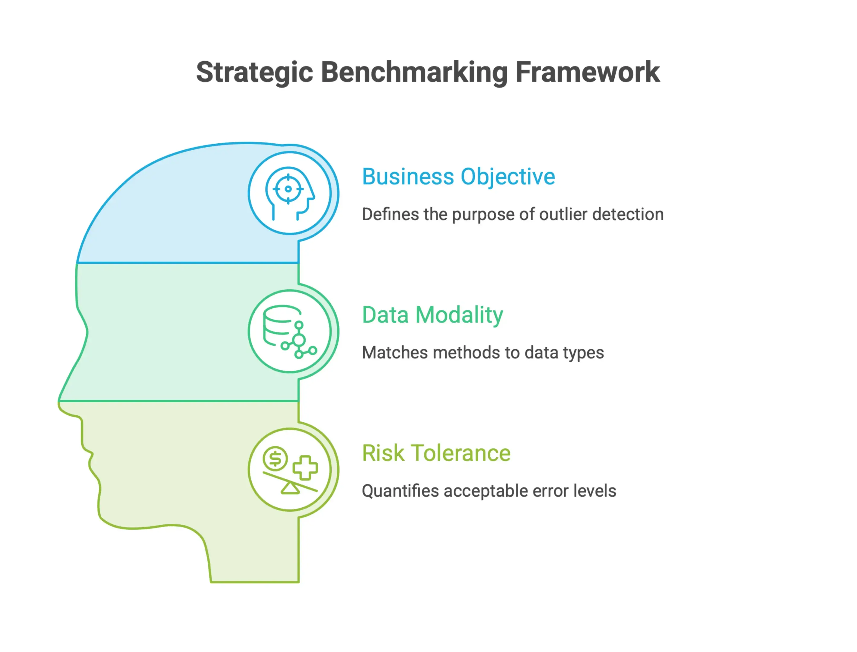
Documenting these three inputs before you run any experiments helps prevent scope creep and keeps the benchmark tied to real operational impact instead of abstract model rankings.

Select Representative Datasets, Metrics, Baselines, and Resource Constraints

Once the objective is clear, the next step is gathering the right evaluation materials. This is where benchmarking efforts often go off track. Teams default to convenient public datasets or lean too hard on accuracy, and neither choice usually reflects production reality.

Datasets should look like the data you expect to process in the real world. Include edge cases, known anomaly patterns from your domain, and data captured under realistic noise conditions. When possible, combine labeled benchmark datasets for controlled comparison with unlabeled production samples for stress testing. That gives you both consistency and realism. Synthetic outliers can also be injected into clean data for controlled benchmarking when you need a repeatable simulation study.

Metrics need to match the risk profile. On imbalanced datasets where outliers are rare, accuracy can be misleading. Precision, recall, F1-score, and area under the precision-recall curve usually tell a more honest story. For ranking-based detection tasks, metrics like average precision score or ROC-AUC can give a fuller view. Choose the primary decision metric before you start testing, not after the results come in. If the goal is to determine which method produces the best ranking of unusual observations, top-k performance is often a better fit because it reflects the alerts human investigators will actually review. The mean value of a benchmark metric should be read alongside its variance, not on its own.

Baselines are essential. Every benchmark should include at least one simple, well-understood reference model. Without one, it is hard to tell whether a more complex method is actually improving results or just adding complexity. Statistical approaches like z-score thresholding or isolation forests often make solid baselines because they are interpretable and relatively lightweight. Practitioners may also use a simple plot to compare baseline behavior before moving to more complex models. When comparing several baseline methods, do not judge thresholding choices by the worst case alone. Nomitech tools can fit naturally into this kind of evaluation workflow when teams want a clearer comparison between methods and a more structured way to track results.

Resource constraints should be part of the benchmark from the start. Inference latency, memory use, training time, and retraining cost all matter in production. A model that looks great on precision but takes hours to retrain on updated data may not be practical at all. Including these constraints ensures the final recommendation can actually be deployed, not just admired on a slide.

Create a Governance Loop for Drift, Retraining, and Continuous Benchmarking

A benchmark done once is a useful start, but it is not the end of the job. Data shifts, business rules evolve, and anomaly patterns change over time. Without a governance loop, even a strong model can quietly lose value in production.

A practical governance loop has three parts:

Drift monitoring should run continuously against the same feature distributions used during benchmarking, and outlier detection should integrate with enterprise data governance frameworks. When incoming data starts to drift away from the training distribution, that is often the first sign that the model’s assumptions are wearing thin. Statistical tests for distribution shift can be automated and tied to alerts, so teams can review issues before performance drops in a meaningful way. This helps address issues early and ensures the model still produces reliable output.

Retraining protocols should be defined ahead of time, not improvised after a problem appears. Set clear rules for when retraining is triggered, what data gets included, and how the updated model is checked before it replaces the current version. That validation step should rerun the same benchmark suite used during initial selection, so every new result is measured against the same standard.

Continuous benchmarking closes the loop by treating model evaluation as an ongoing operational process, not a one-time project. In practice, that can mean a scheduled pipeline that runs the core evaluation suite on a sample of recent production data, compares results with the original baseline, and flags regressions for review. Teams should note governance exceptions and review findings as part of the audit trail. Over time, this builds the kind of audit trail that supports governance, regulatory needs, and vendor accountability. Nomitech’s software can support that ongoing comparison by helping teams keep benchmark results organized and easier to revisit as conditions change.

The end result is a system where the performance claims made during vendor selection stay verifiable throughout the model’s life in production. That kind of traceability is what separates a mature outlier detection program from one that relies on luck and occasional manual checks.

Frequently Asked Questions

Why is benchmarking outlier detection important?

Benchmarking helps teams compare anomaly detection methods under consistent conditions. It supports more reliable decisions by capturing the key benefits of outlier detection in benchmarking, including better data accuracy, clearer inefficiencies, stronger recognition of exceptional performance, and more insightful analysis before deployment. It also gives stakeholders an objective baseline for model comparison and justification.

What makes an outlier detection benchmark reliable?

A reliable benchmark uses representative datasets, validated labels, realistic anomaly types, consistent preprocessing, fair evaluation protocols, and transparent reporting. It should also account for accuracy, variance, and computational cost. Reliable benchmarks should report how summary results were derived and, finally, whether rankings remain stable when protocols change.

Which metrics matter most when evaluating anomaly detection models?

Precision, recall, F1-score, area under the precision-recall curve, ROC-AUC, detection latency, training time, inference time, and memory usage can all matter. The right mix depends on the business cost of false positives, false negatives, and operational delay.

Why does hyperparameter tuning affect benchmark results?

The best hyperparameter settings can vary from one dataset to another, even for the same algorithm. Without per-dataset tuning and clear documentation, rankings may reflect poor experiment design instead of real model performance.

Should teams rely on public leaderboards when selecting a model?

Public leaderboards are useful as a starting point, but they should not be treated as the final answer. Shortlisted methods should be tested on internal or held-out datasets that reflect the actual use case.

Ready to Take the Next Step?

If you’re exploring modern cost estimation platforms, check out Nomitech’s full suite or get in touch with our team to find the right fit for your workflows.

‍